Building Charts

Report Studio offers ten chart types. They share a similar setup, so once you learn one, the rest are easy. This page covers the common concepts first, then each chart type in detail. A chart reads whichever data source you picked when you created the report, and the source decides what the Group By and Value steps offer. The walkthroughs below describe the Estimating source. For the Risk Register, see Charts on the Risk Register source.

This page is part of the Report Studio guide.

Concepts shared by all charts

The wizard

Chart setup is a short wizard of collapsible steps. Each step header shows a status badge:

Required (red): you must complete this step.
Complete (green): the step is done.
Optional (gray): you can skip it.

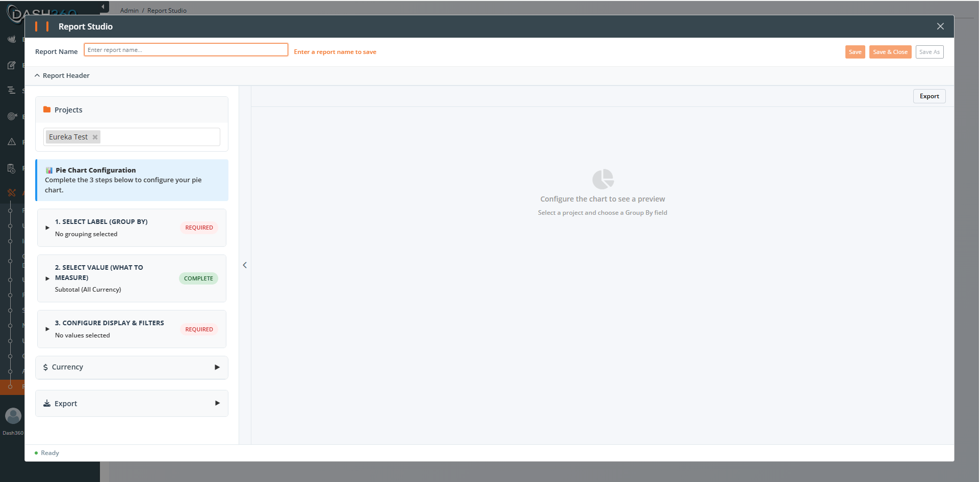
Click a step header to open or close it. The preview updates as you go.

A chart wizard showing the collapsible steps with Required and Complete badges

Group By (the category or series)

Every chart needs something to group by. You choose a field such as WBS (with an inline Level 1 to 6 selector), Resource Level (with its own Level 1 to 6 selector), CAM, Cost Class, Cost Set, Resource Type, or any dynamic field. Each unique value becomes a slice, bar, line, or panel. Cost Set appears only after you have selected a project, and only when that project defines cost sets.

Grouping by Cost Set

A cost set is a named basket of cost classes, and the same cost class can belong to more than one set. A report grouped by Cost Set therefore counts a shared class once in every set that holds it, so the buckets add up to more than the project. This is the honest answer to the question “what is in each set?”, but it means the usual reading of a total does not apply. Two things happen automatically when the project’s sets overlap:

A caution note appears under the chart naming the classes that are counted more than once. On a pie or doughnut it also names the figure the percentages are shares of, which is the drawn total rather than the project total.
The grand total row is withheld from the data table, because a spreadsheet exported from the report outlives the note that explains the number.

Both are controlled from Display Options:

Option	Default	What it does
Note when cost sets overlap	On	Shows the caution note under the chart
Keep the grand total when sets overlap	Off	Restores the grand total row in the data table

The two are independent: you can keep the note and the total, drop either, or drop both. If the project’s sets do not share any cost class, nothing overlaps, no note appears, and the grand total behaves as it does on any other grouping.

Using Cost Set as a filter rather than a grouping does not double count anything. A filter narrows the rows to the classes in the sets you pick, so the totals stay comparable with the rest of the report and no note appears.

Value Type (what to measure)

You then choose what to measure:

Subtotal (All Currency Resource Results): sum all currency values.
Specific Resource Result(s): pick particular resource results from a tag box.

That is the Estimating wording. Another source asks for one of its own named measures instead: see Value to plot for the Risk Register.

Time period (trend and time-based charts)

Charts that show data over time let you pick the time axis: fiscal year, monthly, or a calendar period. Two helpers appear depending on your choice:

Smart Monthly: when you choose monthly, set how many months to show and where the window starts.
Calendar Unassigned: when you choose a calendar period, decide how to label periods outside the defined ranges.

A Risk Register chart plots against one of the register’s own dates instead, because a register has no reporting period: see Time axis.

Filters

Every chart has a Filters section. By default, Resource Type is set to Labor, Non-Labor, and Travel. Add filters to focus the chart.

Series options (color, caption, visibility)

Where a chart has multiple series or categories, you can set each one’s color, edit its caption, and show or hide it, with Select All / Unselect All helpers.

Number formatting

Every value carries the formatting its own measure calls for, in the axis, the point labels, the tooltip, and the data table alike:

The measure is	It reads
Money (Item Cost, cost exposure)	Currency symbol and the K or M scale: `$400.00K`
A count (Risks, Response Actions)	Whole numbers, no symbol and no scale: `23`
A duration in days (schedule exposure)	A day marker: `43.07 d`
An index (SPI, CPI)	Two decimals, so 1.06 and 1.10 stay distinct
A percentage (Earned %)	A percent sign: `10.00%`

A measure can withhold the currency symbol but never add one back, so turning Show Currency Symbol off still hides it on money.

Data table headers

Where a chart has a data table, you can rename its column headers. Leave an input empty and the header keeps the wording Dash360 derives from the field you grouped by; each input’s placeholder shows you that wording before you replace it.

A Pie or Doughnut table (Standard style) has a fixed set of columns, so all four are nameable: Label header, Value header, Percent header, and Records header. The last three appear only while their column is switched on.
Every other chart table puts a time period in each column after the first, so only the first is nameable: Series Header.

Group values into named series

Sometimes several values of your Group By field belong together on the chart. A dozen engineer resource codes that should read as one “Engineers” line, or two cost classes that should be plotted as a single combined total. Grouped series does this: the values sharing a name are added together and the chart draws one series where it drew several. The control sits in the Group By step, under the field list. Click Group values to open the Group Series window. It has two tabs.

Build: tick the values

The Build tab lists every value the report currently returns. Tick the ones that belong together, type a name at the bottom, and click Create series. The grouped values stay in the list, greyed out, labelled with the group they went to, so you can always see where a value ended up. What the chart will show at the right lists your groups and the values that stayed on their own, which is the whole answer before you save anything. When the values you ticked share an opening run of characters, a checkbox offers to match on that run instead of on the exact values:

Also include values starting 420128, including ones added later

Leave it off and the group holds exactly what you ticked. Turn it on and a value added to the project next month joins the group on its own, with no change to the report. The label tells you how many values already in the list the prefix would also take, so you can see the reach before you accept it.

Rule: write it yourself

Everything the Build tab produces is a formula, and the Rule tab shows it. A rule reads one field and returns the series name a value should be plotted under, not a number:

SWITCH(TRUE,
  STARTSWITH([Resource Code], 'L.EN'), 'Engineers',
  STARTSWITH([Resource Code], 'L.SC'), 'Scientists',
  [Resource Code])

Read it as: if the resource code starts L.EN plot it as “Engineers”; if it starts L.SC plot it as “Scientists”; otherwise keep the code’s own name. Patterns below the box write a worked example using this project’s own values, and the insert buttons add a field reference or a function without typing it. Two points worth understanding:

The last argument is the fallthrough. It is what a value gets when it matches nothing. Ending the rule with the field reference, as above, means unmatched values keep their own names. Put 'Other' there instead and every unmatched value collapses into a single “Other” series.
Conditions are tried in order. The first one a value matches wins, so a value reaches one group and one only. Put the narrow condition above the broad one.

Result below the box lists what the rule produces, and flags a rule that reads a field the chart does not have, quotes a bare word, or writes a branch nothing can reach. Editing the formula by hand takes over from the tick list: the Build tab then shows the rule as authored here rather than pretending a list describes it. Click Done to apply, Cancel to discard. What follows the group: colors, ordering, captions, show/hide, the chart data table, and the Excel export all apply to the group, not to the values inside it. The group is a single series as far as the rest of the chart is concerned. Remove the grouping and the individual values come back.

A grouped series has no code file entry behind it, so the Show values as setting (Code, Description, or Code + Description) does not apply to it. The name you gave it is shown as-is. Values that keep their own names still follow that setting.

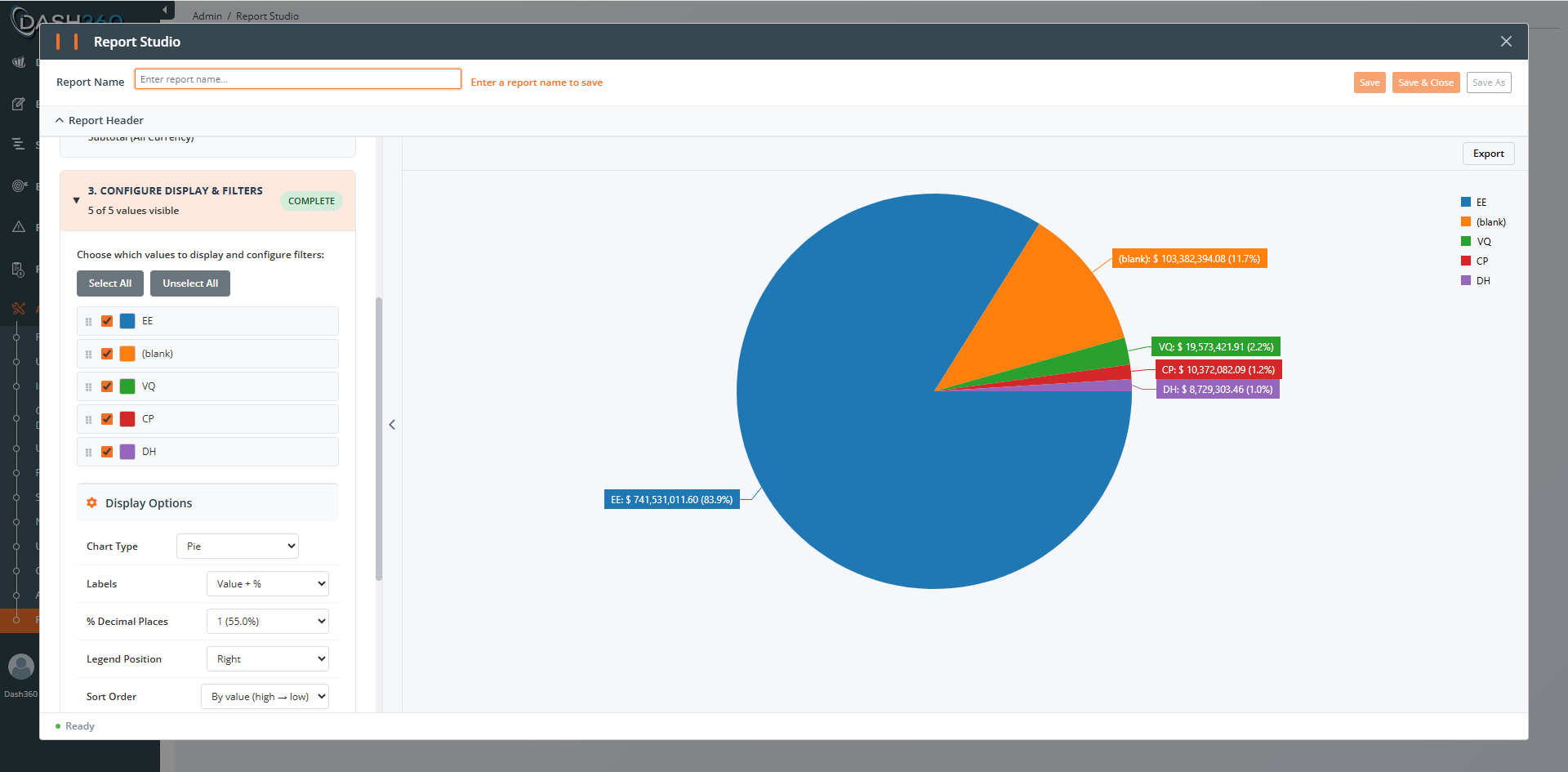
On a Pie or Doughnut chart, grouping is unavailable if the report carries the Average FTE over months setting. That option divides each slice by the number of months that slice spans, so two already-divided slices cannot be added together correctly. The pie’s own display options do not offer that setting, so a pie only carries it when the report was imported or built elsewhere; use a Bar, Stacked Bar, Line, or Trellis chart, where the division is per time period and grouping stays correct.

Grouping adds values together, so it covers “show these two cost classes as one line”. What it cannot do is subtract or divide them: a variance or a ratio is not a group. Use a calculated field for those.

Pie and Doughnut

Best for showing proportions of a whole, for example cost share by Resource Type. A Doughnut is a Pie with a hollow center. Steps: 1. Select Label (Group By), 2. Select Value, 3. Configure Display & Filters. Display options:

Option	Choices	Notes
Chart Type	Pie, Doughnut
Inner Radius	10% to 90%	Doughnut only; controls hole size (default 50%)
Labels	Value + %, % only, Value only, None	Default Value + %
% Decimal Places	0 to 4	Decimal places for every percentage (slice labels, tooltip, and data table). Default 1. Increase it so tiny slices show their real value (e.g. 0.01%) instead of rounding to 0.0%
Legend Position	Bottom, Right, Left, Top, Hidden	Default Right
Sort Order	By value (high to low), By value (low to high), Alphabetical	Default high to low
Group Small Values	Off, below 1%, 2%, 3%, 5%, 10%	Combines tiny slices into one “Other” slice
Include Data Table	On / Off	Shows a table beneath the chart. When on, choose a Style: Standard or Time-phased (see below)
Data Table Style: Standard	Default	The classic table: one row per slice. Choose which columns appear (Value and % show by default, Records is off by default; the group-by label column is always shown) and toggle Show Total Row
Data Table Style: Time-phased	Optional	One row per slice with a column per time period. Choose the Time Period (Fiscal Year, Monthly with a month-range picker, or a Calendar Period), and toggle Show Column Grand Total (a Total column on the right; each slice’s total matches its pie value) and Show Row Grand Total (a Total row at the bottom with per-period totals), each with an optional caption. Both totals show by default

Use Group Small Values when a pie has a long tail of tiny slices. It keeps the chart readable by rolling small slices into one. Note that the Time-phased table lists every slice individually; small values are not grouped there.

The data table sits beneath the chart and scrolls with the report, so a grouping with many values shows every row and the grand totals. Exporting the report to Excel follows whichever table style and totals are selected.

Pie and Doughnut display options: chart type, inner radius, labels, legend, sort, and group small values

Bar Chart

Best for comparing a single value across categories, for example cost by CAM. Category-based, with no time dimension. Steps: 1. Select Category (Group By), 2. Configure Display. Display options:

Option	Notes
Fit Width To Content	On by default. Sizes the chart to the width its own category labels need, so a handful of categories stays compact instead of stretching across the page. Turn it off to go back to the full-width layout
Legend Position	Bottom, Right, Left, Top
X-Axis Title / Y-Axis Title	Text labels for the axes
X/Y Axis Title Color	Color pickers
Show X Axis	Toggle the horizontal axis
Show Value Labels on Bars	Print the value on each bar
Show Percentile Line	Draw a reference line at a percentile (P50 median, P75, P90, P95, P99, or Max)
Show Percentile Value Label	Label the percentile line with its value

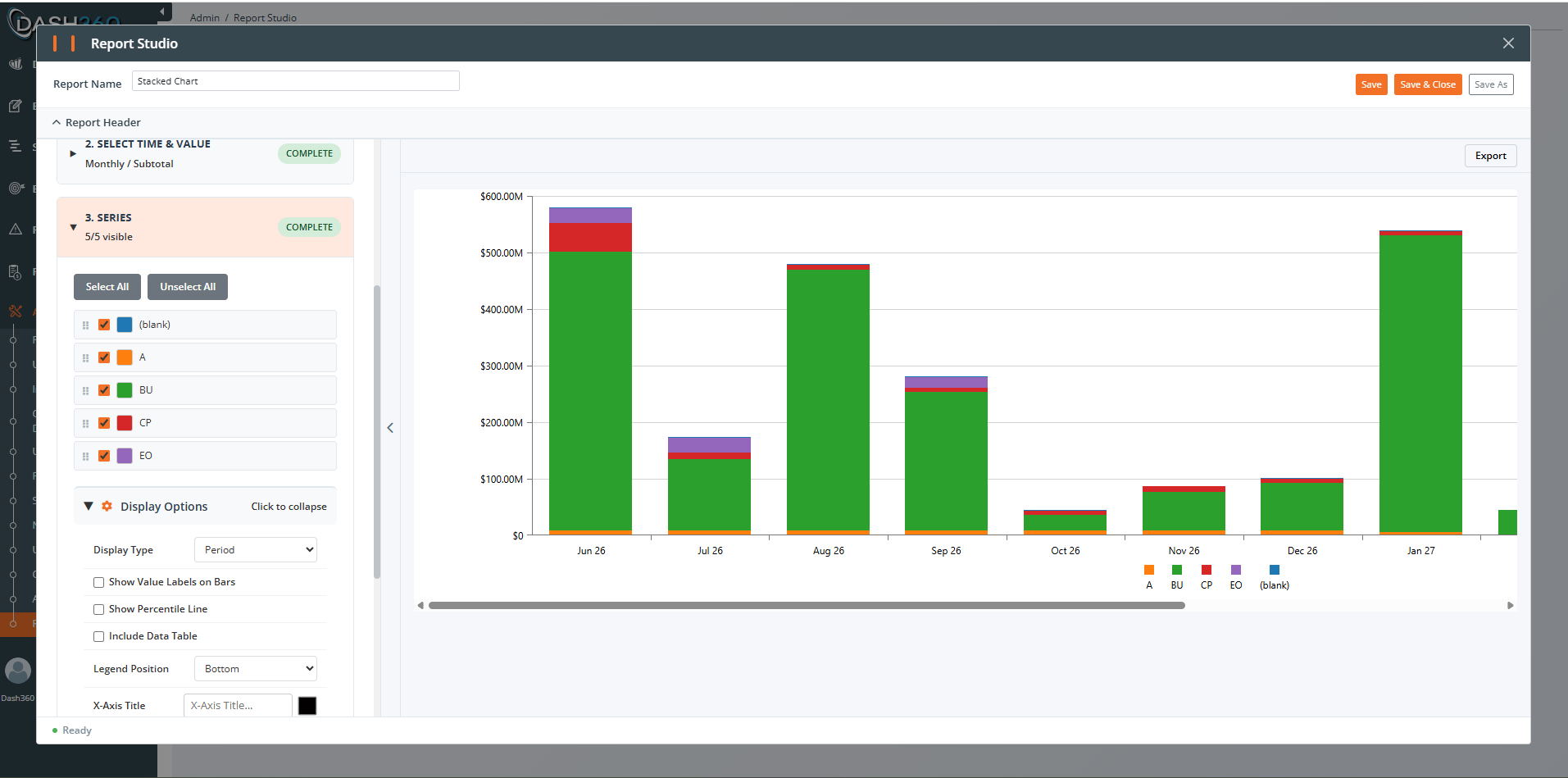
Compares several series next to each other across categories. Shares its setup with the Stacked Bar; the difference is that bars sit beside each other instead of stacking. Steps: 1. Select Group By, 2. Select Time & Value, 3. Series. See the Stacked Bar options below; they are the same.

Stacked Bar

Shows part-to-whole relationships across categories or time, with series stacked into one bar. Steps: 1. Select Series (Stack By), 2. Select Time & Value, 3. Series. Display options (Step 3):

Option	Notes
Display Type	Period or Cumulative
Show Value Labels on Bars	Print the value on each segment
Show Percentile Line + Value Label	Reference line at P50 to Max
Show Fiscal Year Prefix on Year Labels	Auto when projects match; a toggle when fiscal and calendar projects are mixed
Include Data Table	Shows a table beneath the chart, with: Show Column Grand Total, Column Total Caption, Show Row Grand Total, Row Total Caption
Fit Width To Content	On by default. Sizes every column to the widest value it holds, and matches the bars to those columns, so a report with a few time periods stays compact instead of stretching across the page. Turn it off to go back to the full-width layout

Cumulative display turns a period chart into a running total, which is the basis of an S-curve view of spend over time.

Turning Include Data Table on also switches Show X-Axis Labels off and moves the legend to the top. The table column headers already name every period, so the axis labels repeat them; and a legend along the bottom would sit between the chart and the table it belongs to. Both are ordinary settings afterwards, so you can change either back. Turning the data table off again restores what was there before.

Fit Width To Content keeps one standard width for every value column: the widest value in the report sets it, and the bars line up with it. All the columns share that width, because each bar has to sit directly over its own column. A chart sized this way also copies into PowerPoint at its natural size, so it stays sharp instead of being scaled down.

Stacked Bar setup: time period with Smart Monthly controls and the Step 3 display options

Line, Spline, and Area

Track cost over time. Line uses straight segments, Spline uses smooth curves, and Area fills under the line. The chart type is set when you create the report; the setup is otherwise identical. Steps: 1. Select Series (Group By), 2. Select Time & Value, 3. Series. Display options (Step 3):

Option	Notes
Show Data Points	Markers on the line (default on)
Point Size	4, 6, 8, 10, or 12 px
Line Width	1 to 5 px
Display Type	Period or Cumulative
Show Value Labels on Points	Print values at each point
Show Percentile Line + Value Label	Reference line at P50 to Max
Show Fiscal Year Prefix on Year Labels	Auto or toggle, as above
Include Data Table	With column/row grand totals and captions, as above
Fit Width To Content	On by default; sizes the chart and table to their content, as above

Combo Chart

Draws a bar layer and a line layer on one shared time axis. It is the shape most earned value and budget reporting wants: what each period spent, drawn under where the project stands to date. The two layers are independent. Each chooses what it measures and whether it shows each period on its own or a running total to date, which is what a single chart type cannot do. Steps: 1. Bars, 2. Lines, 3. Time Axis, 4. Series, 5. Display Options.

Start from a template

A new Combo Chart offers ready-made charts for your data source. Pick one and the whole chart is configured, ready to save; take it apart afterwards, or ignore the templates and build your own.

Template	Source	What it draws
Earned Value Performance	Cost Performance Report	Period planned, earned and actual as bars, under the cumulative curves, against Budget at Completion
Budget vs Actual	Estimating	Actuals to date stacked by WBS Level 2, under the cumulative budget curve

The templates only appear while the chart is still empty, because applying one to a chart you have started would discard your work.

The bar layer (Step 1)

Bars show one of two things:

Several measures, drawn side by side or stacked.
One measure, split by a field such as WBS (with the same inline Level 1 to 6 selector the other charts use), Cost Class or CAM. Stacked, those bars add up to the measure’s total, so a line of the same measure sits exactly on top of the stack.

The line layer (Step 2)

Curves drawn over the bars. Cumulative values belong here: they are read at the reporting period, never summed. The line layer can also be split by a field, or left as Nothing, which draws one line of the value itself. That single line is the total a stack of bars adds up to.

Cost Class per layer (Estimating)

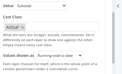
On the Estimating source, each layer has its own Cost Class, set in the Bars and Lines steps rather than in Filters. This is what lets one chart draw budget against actuals. Estimating reports one cost subtotal, so cost class is not a way of narrowing the rows, it is what makes an amount budget, actual or committed. Set Cost Class to Actual on the bars and Budget on the lines and the chart compares the two. Every other filter (WBS, Work Package, CAM, Resource Type, Fiscal Year) stays in Filters and applies to the whole chart, because it is scope and both layers answer it the same way.

A layer’s own Cost Class wins over the one in Filters, and the step says so when you have set both. That order matters: the layer’s choice is what the series IS, and its caption says so, so letting a chart-wide filter override it would relabel your data.The same holds for a filter applied while reading the report, including a dashboard’s filter strip. Narrowing Cost Class there does not change a layer that sets its own, because it would turn a budget curve into a second actuals curve still labelled Budget. Every other filter reaches both layers as you would expect.

Value axis (Step 4)

Each series is drawn against a value axis, decided automatically: anything whose format differs from the bars’ gets its own right-hand axis. Money bars with an SPI or CPI line is the case this exists for. An index sits around 1.00, and against an axis scaled to hundreds of millions it would be a flat line along the floor. When every series is money, there is one axis and the control reads Auto (left) throughout. You can override any series to Left or Right. Reference draws a series broken rather than solid, marking it as the line the others are read against. Budget at Completion and a budget curve are what it is for.

Data table

One table beneath the chart, in sections: the bars under their heading, then the lines under theirs. You can rename both headings in Display Options. The Total column adapts to what a row means. Period rows are summed across the periods; cumulative rows are read at the reporting period, because a running total is already the total and adding it up period by period would count the opening months over and over.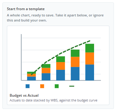

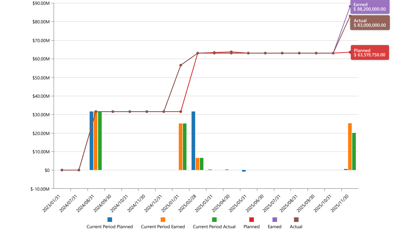
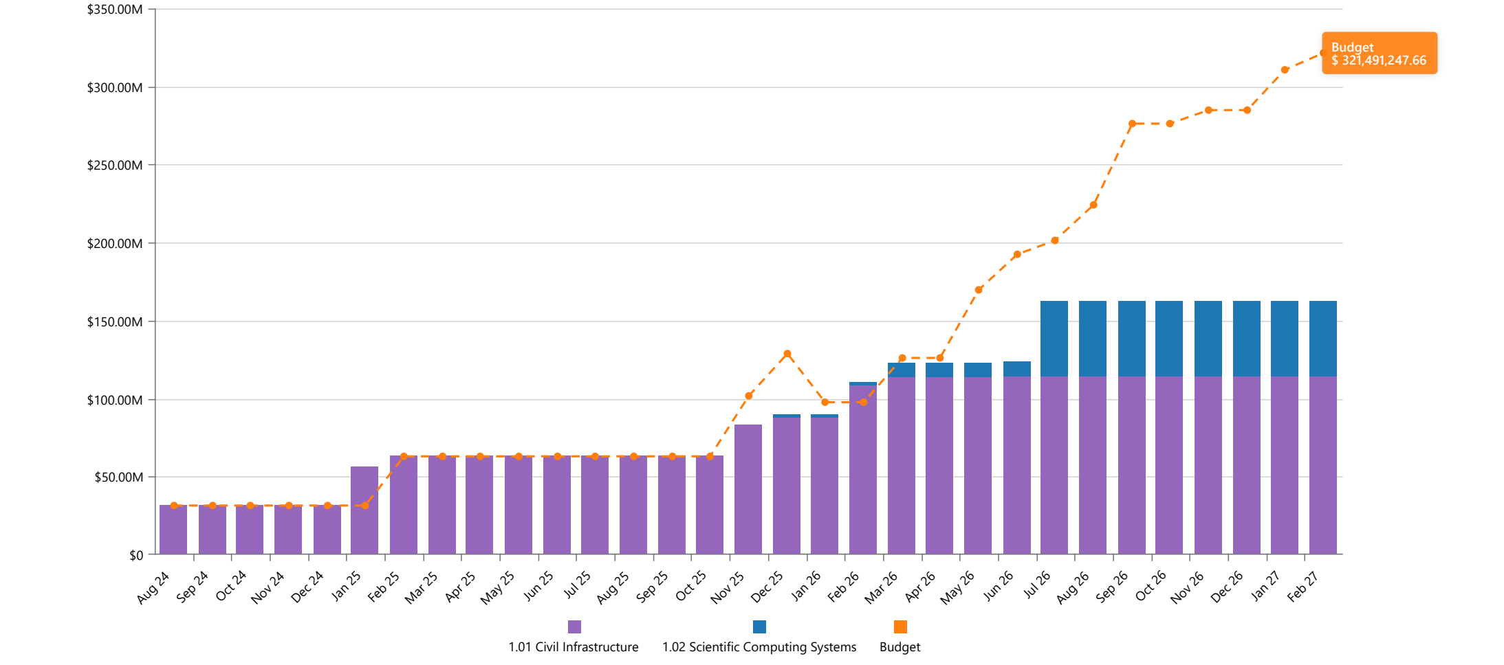
The Combo Chart template step offering Earned Value Performance and Budget vs Actual

The Bars step with Cost Class set per layer, beside Value and the running-total option

An earned value performance combo: period bars under cumulative curves with a broken budget line

A Budget vs Actual combo: actuals stacked by WBS under the budget curve, with its sectioned data table

Two money axes mislead. Putting one money series on the right-hand axis gives it a scale of its own, and the eye still compares heights. A WBS element peaking at

554,001.43 moved to its own axis was drawn nearly as tall as a

243M budget curve, because its axis stopped at $600,000. Use the second axis for a different unit, an index or a percentage, not for more money.

A stacked bar’s axis is fixed, and the control is disabled for it. Bars can only stack when they share an axis, so moving one member to the right would take it out of the stack and draw it beside the others against a scale nothing else uses. Reference is likewise offered on curves only: drawing a bar broken marks a block of a stack as though it were a line.

Period bars under a cumulative line are not comparable. The bars are one month and the curve is everything to date, so the bars stay small and the chart cannot answer “are we under budget”. If that is the question, set the bars to a running total as well.

The Budget vs Actual template is not a copy of the standalone Budget vs Actual report. That report adds commitments into the same bars without cumulating them, which one layer cannot reproduce. Use the template for the shape and the budget comparison; use the standalone report when you need its exact commitments treatment.

Trellis (small multiples)

Draws one small chart per group value and lays them out side by side, so you can compare the same pattern across many groups. Each unique value of the Group By field becomes its own chart. Steps: 1. Select Rows (Group By), 2. Select Time & Value, 3. Chart Type & Display. Display options (Step 3):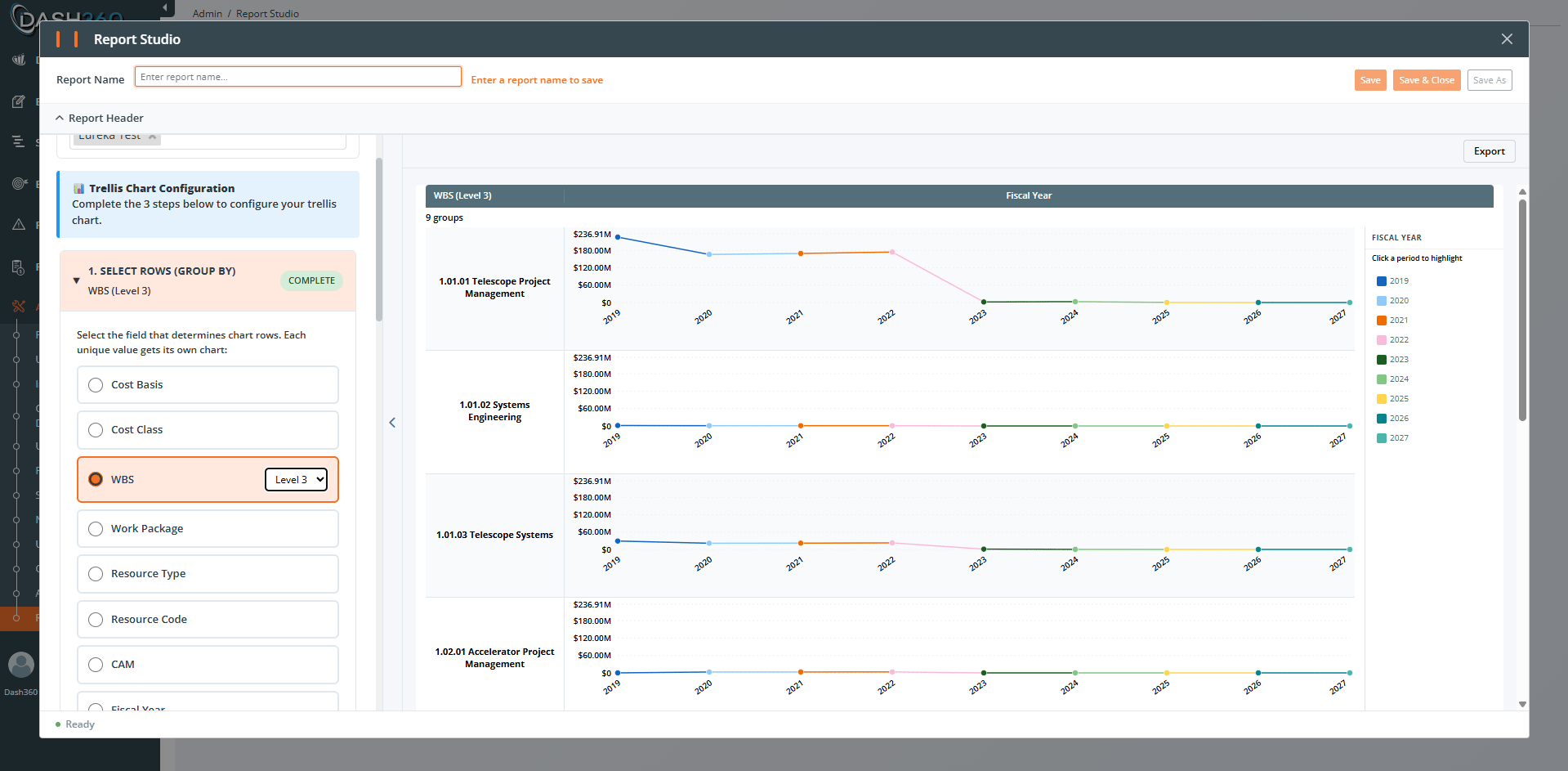

Option	Notes
Chart Type	Line, Spline, Scatter, or Bar (per-panel chart style)
Series Captions	Custom caption per series, with Reset Captions
Display Type	Period or Cumulative
Legend	Hidden, Bottom, Right, Top
Row Height	100 to 300 px per panel row

Trellis display options: chart-type pills and the row-height slider

A Group By field with many unique values produces many panels. Filter the group, or pick a higher WBS level, so the trellis stays readable.

Charts on the Risk Register source

A Risk Register chart follows the same wizard as any other, with the differences below. Every chart type is available, Trellis included.

Scope, in place of snapshots

A Risk report reads one project’s live register rather than a set of snapshots, so the scope panel asks for two things instead:

WBS: name a node and the chart shows the risks on it and everything beneath it. Leave it empty for every WBS.
Statuses: Active and Proposed are ticked to begin with. A register keeps its own history, so leaving the retired, realized, and deprecated rows in can make a project look considerably worse than it is.

Group By

Group by any register dimension: Status, Classification, Risk Register Category, Type, Handling Strategy, Owner, Assignee, or WBS with an inline Level 1 to 9 selector. Where a grouping carries both a code and a description, Show values as offers three readings of it:

Choice	Reads
Code + Description	`CS016.1.P1.OM.01 Project Management (PM)`
Code	`CS016.1.P1.OM.01`
Description	`Project Management (PM)`

A chart usually wants Description, because a WBS code carries its whole path and crowds the label out. The data table below the chart has its own Values as control, so the table can carry the full code while the chart stays short.

Value to plot

Six measures are offered:

Measure	What it totals
Risks	How many risks fall in the group
Response Actions	How many response actions those risks carry
Total Cost Exposure, before and after response	Cost impact times likelihood
Total Schedule Exposure, before and after response	Schedule impact times likelihood, in days

The two exposure pairs are named with your project’s own wording for a risk before and after its response actions, so they may read differently in your registry (for example, “Risk Total Cost Exposure” alongside “Mitigated Total Cost Exposure”).

Cost impact, probability, rank, and the three point estimates are deliberately not offered. Exposure adds up across a group because impact times likelihood is an expected value. A probability does not: summing eight probabilities of 0.8 gives 6.4, and the average of two ranks is not a rank. Those stay columns of a Flat Data Grid, where each value sits on its own row and is never summed.

Time axis

A register is live, so it has no reporting period and no fiscal year to plot against. The charts that need a horizontal axis (Stacked Bar, Side-by-Side, Line, Spline, Area, and Trellis) use one of the register’s own dates instead, bucketed into periods:

Dates: Trigger Date, Start Date, Finish Date, Last Updated, Last Reviewed.
Grain: Monthly, Quarterly, or Yearly.

A new chart starts on Trigger Date (Monthly).

A risk with no date in the chosen field is left out of a date axis rather than bucketed under a blank period. A risk with no value in the chosen grouping is kept and shown as (Unassigned), so the chart still totals to the register’s own figure.

Pitfalls to avoid (all charts)

Too many categories. Pies with dozens of slices and bar charts with dozens of bars are hard to read. Filter, group small values (pie), or pick a higher WBS level.
Forgetting the Value Type. If a chart looks empty or wrong, confirm whether you meant Subtotal (all currency) or specific resource results.
Mixing Budget, Actual, and Earned in one series unintentionally. If you do not filter Cost Class, a single bar or slice can blend them. Filter Cost Class, or split values with calculated fields.
A grouping rule with no fallthrough. If a rule’s last argument is a fixed name rather than the field reference, every value that matches nothing lands in that one series. Check the Preview before saving.
Default Resource Type filter. Charts start filtered to Labor, Non-Labor, and Travel. If a category is missing, check this filter.
Cumulative vs Period confusion. Cumulative shows a running total; Period shows each period on its own. Pick deliberately.

​Building Charts

​Concepts shared by all charts

​The wizard

​Group By (the category or series)

​Grouping by Cost Set

​Value Type (what to measure)

​Time period (trend and time-based charts)

​Filters

​Series options (color, caption, visibility)

​Number formatting

​Data table headers

​Group values into named series

​Build: tick the values

​Rule: write it yourself

​Pie and Doughnut

​Bar Chart

​Side-by-Side Bar

​Stacked Bar

​Line, Spline, and Area

​Combo Chart

​Start from a template

​The bar layer (Step 1)

​The line layer (Step 2)

​Cost Class per layer (Estimating)

​Value axis (Step 4)

​Data table

​Trellis (small multiples)

​Charts on the Risk Register source

​Scope, in place of snapshots

​Group By

​Value to plot

​Time axis

​Pitfalls to avoid (all charts)

​Where to go next

Understanding Your Data

Calculated Field Cookbook

Building Charts

Concepts shared by all charts

The wizard

Group By (the category or series)

Grouping by Cost Set

Value Type (what to measure)

Time period (trend and time-based charts)

Filters

Series options (color, caption, visibility)

Number formatting

Data table headers

Group values into named series

Build: tick the values

Rule: write it yourself

Pie and Doughnut

Bar Chart

Side-by-Side Bar

Stacked Bar

Line, Spline, and Area

Combo Chart

Start from a template

The bar layer (Step 1)

The line layer (Step 2)

Cost Class per layer (Estimating)

Value axis (Step 4)

Data table

Trellis (small multiples)

Charts on the Risk Register source

Scope, in place of snapshots

Group By

Value to plot

Time axis

Pitfalls to avoid (all charts)

Where to go next